Physics in flight simulators
DRT 112 Applied Physics for Aircraft Technology
Lesson
By the end of this module you will be able to
- Describe the parts of a flight simulator: state, force model, integration, sensors and controller
- Step motion forward with the Euler method and explain the effect of time-step size
- Use a drag model to find terminal velocity
- Explain the difference between SITL and HITL
- Identify why simulation results differ from real flight and how to validate a model
Why fly in a simulator first
Testing new software or a new mission on a real drone is risky. A mistake can crash the drone, damage it or endanger people. A flight simulator lets you try things any number of times with no risk: training pilots, testing autonomous missions and tuning control systems.
But a simulator is only as accurate as the physics inside it. This module opens it up to see what it computes, using Modules 1–4 and the calculus from DRT 111.
What a simulator computes
A simulator runs a loop hundreds to thousands of times per second.
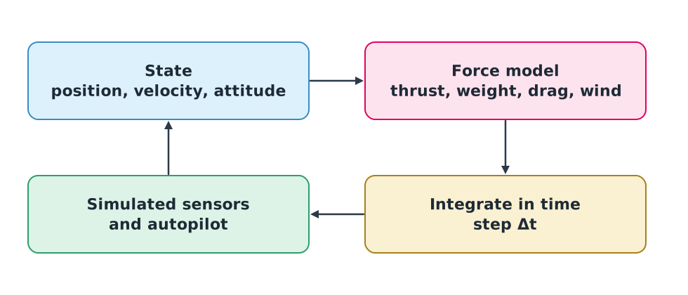
- State holds the current position, velocity, attitude and rotation rates.
- The force model computes all forces and moments from the current state: thrust, weight, drag and wind.
- Integration in time uses Newton’s second law to find acceleration, then computes the new state after .
- Simulated sensors and autopilot produce what the IMU, GNSS and barometer should read, with noise. The autopilot computes new motor commands and the loop returns to step 1.
Stepping forward with the Euler method
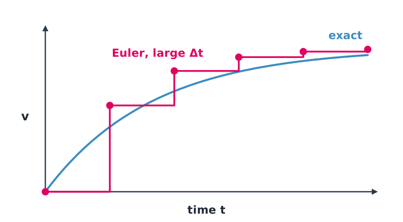
The simplest method is the Euler method, which assumes acceleration and velocity stay constant over a short interval :
Example 1. Simulating a climb by hand
A 2 kg drone with 22 N of thrust starts at rest on the ground. Ignore drag and use s.
Acceleration m/s², constant.
| Step | Time (s) | (m/s) | (m) |
|---|---|---|---|
| 0 | 0.0 | 0.000 | 0.0000 |
| 1 | 0.1 | 0.119 | 0.0000 |
| 2 | 0.2 | 0.238 | 0.0119 |
| 3 | 0.3 | 0.357 | 0.0357 |
The exact answer from at s is 0.0536 m. The Euler method comes out low because it uses the velocity at the start of each interval throughout the interval. Reducing reduces the error.
Key idea
A time step that is too large makes simulation results inaccurate and can even make values oscillate and blow up, especially for fast dynamics like a drone’s rotation. Real simulators therefore compute physics at high rates and often use integration methods more accurate than Euler.
Drag and terminal velocity
Air drag on a whole drone can be approximated by
where is the effective drag area. As an object falls, drag rises with speed until it equals weight and speed stops increasing. This is the terminal velocity:
Example 2. If the motors stop in flight
A 2 kg drone has m²:
That is about 91 km/h. The figure helps assess how severe a fall would be, and it is one input to ground-risk assessment in DRT 431.
SITL and HITL
| Type | Where the autopilot runs | Used for |
|---|---|---|
| SITL (Software In The Loop) | The real autopilot software runs on a computer | Testing missions, flight modes and new code quickly, with no hardware |
| HITL (Hardware In The Loop) | A real flight-controller board, fed simulated sensor data by a computer | Testing firmware on real hardware and checking processing timing |
Both ArduPilot and PX4 include SITL and connect to 3D simulators such as Gazebo. You will keep using SITL in DRT 226, DRT 334 and DRT 335.
When simulation and reality disagree
The gap between simulation and reality has several causes:
- Thrust and efficiency curves in the model do not match the real motors and propellers.
- Battery voltage sag, covered in Module 4, is often not modelled.
- Gusts and turbulence are more complex in reality.
- Ground effect: within about one rotor diameter of the ground, thrust increases.
- Sensor noise and delay differ from the settings.
To validate a model, compare flight logs from simulation and real flight on the same mission: hover power, climb rate and response to commands. Then adjust the model parameters to bring them closer.
Module lab
In class (see lab L14 in the knowledge base)
- Run ArduPilot or PX4 SITL as directed by your instructor. Take off, hover at 10 m, then climb at a constant rate.
- Extract current, voltage and altitude from the log; calculate hover power and climb rate.
- Compare with your hand calculations from Modules 3 and 4 and explain the differences.
- If a real drone is available in the lab, fly the same mission and compare all three: calculation, simulation and real flight.
Common mistakes
Watch out
- Trusting simulation without checking against reality.
- Using too large a time step, giving inaccurate or unstable results.
- Ignoring drag when estimating fall speed, which gives far too high a value.
- Assuming passing SITL means ready to fly. Test in stages, starting in a safe area at low height.
Summary
- A simulator loops through state, forces, integration, and sensors with a controller.
- The Euler method computes and ; smaller steps are more accurate.
- Drag and terminal velocity .
- SITL runs the software on a computer; HITL uses real hardware with simulated sensors.
- Always validate simulation results against real flight logs.
Check your understanding
- A 1 kg drone has 12 N of thrust, ignoring drag. What is its vertical acceleration?
- Using Euler with s and the acceleration from question 1, find the velocity at s.
- If doubles, by what factor does terminal velocity change?
- To test firmware on a real flight-controller board without flying, would you use SITL or HITL?
- Give two reasons why simulated flight time might be longer than real flight time.
Answers
- m/s²
- m/s (constant acceleration, so it matches the exact value)
- HITL
- For example: the model ignores battery voltage sag, has no gusts, or uses unrealistically high motor efficiency
Key formulas
| Vertical acceleration | |
| Euler method | |
| Drag | |
| Terminal velocity |
Key references
- ArduPilot Dev Team. SITL simulator (software in the loop). link
- PX4 Autopilot. PX4 user and developer guide. link
- Beard, R. W., & McLain, T. W. (2012). Small unmanned aircraft: Theory and practice. Princeton University Press.
- Serway, R. A., & Jewett, J. W. (2018). Physics for scientists and engineers (10th ed.). Cengage.
Further reading
Study the assigned knowledge units in advance, review media and take the module quiz
Physics and assessing realism
Interpreting endurance test results
From aerodynamic results to DroneSim: preparing force tables
Planning CFD work: from problem to credibility evidence
Channel-flow lab: analytic solution versus numerical methods
In class / field
Lab or field practice from worksheets with a safety checklist
Learning evidence: Checked worksheets and quiz results