Module 5/5 · Weeks 13–15 · 27 h

Elementary calculus of motion

DRT 111 Applied Mathematics for Technology

About 90 minDraft, awaiting reviewLast updated 26 September 2026

By the end of this module you will be able to

Explain the derivative as a rate of change and as the slope of a tangent line
Differentiate polynomials with the power rule and find maxima and minima
Estimate velocity from flight-log position data with finite differences
Explain the integral as the area under a graph and estimate it with the trapezoidal rule
Calculate charge consumed and explain the drift that comes from integrating IMU data

Prerequisites: DRT 111 Module 1 (functions and graphs)

The mathematics of change

Every number in a flight log changes over time. Altitude rises, the battery drains, speed wobbles in the wind. The important questions are not only “what is the value now?” but also “how fast is it changing?” and “how much has built up so far?”

Calculus answers these with two tools. The derivative gives the rate of change at an instant. The integral gives the total accumulated over an interval. The two are inverses of each other. This module focuses on understanding and on calculating with real data rather than on formal proofs.

Rate of change and the derivative

Average velocity

If a drone is at position $x_{1}$ at time $t_{1}$ and at $x_{2}$ at time $t_{2}$ , its average velocity is

\overset{v}{ˉ} = \frac{Δ x}{Δ t} = \frac{x _{2} - x _{1}}{t _{2} - t _{1}}

On a position–time graph this is the slope of the straight line through the two points.

Instantaneous velocity

If we shrink the interval $Δ t$ towards zero, the line through two points becomes a tangent that touches the graph at a single point. Its slope is the instantaneous velocity, called the derivative of position with respect to time:

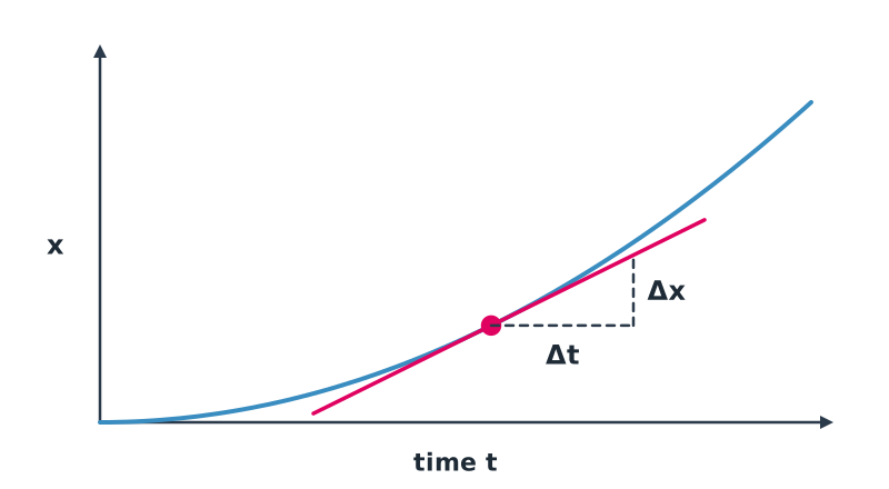
v (t) = \frac{d x}{d t} = Δ t \to 0 lim \frac{x ( t + Δ t ) - x ( t )}{Δ t}

Position–time curve with a pink tangent line at one point and a small triangle showing delta t and delta x — Figure 1. The slope of the tangent to the position graph is the velocity at that instant

Likewise, the derivative of velocity is acceleration, $a = d v / d t$ .

The power rule

You do not have to compute a limit every time. For polynomials, use the power rule:

\frac{d}{d t} t^{n} = n t^{n - 1}

together with two simple rules: the derivative of a constant is zero, and the derivative of a sum is the sum of the derivatives.

Example 1. Position, velocity, acceleration

A drone accelerates horizontally with position $x (t) = 5 t^{2}$ metres.

Velocity $v (t) = \frac{d}{d t} (5 t^{2}) = 10 t$ ; at $t = 2$ s, $v = 20$ m/s
Acceleration $a (t) = \frac{d}{d t} (10 t) = 10$ m/s², constant throughout

Finding maxima and minima

At the highest or lowest point of a smooth graph the tangent is horizontal, so the derivative is zero. We can use this to find maximum values.

Example 2. Maximum height

An object launched upward has height $h (t) = 12 t - 1.5 t^{2}$ metres.

$\frac{d h}{d t} = 12 - 3 t = 0 \Rightarrow t = 4$ s
Maximum height $h (4) = 12 (4) - 1.5 (16) = 48 - 24 = 24$ m

Derivatives from real data

Flight-log data are samples in time, not formulas, so we estimate derivatives with finite differences:

v_{k} \approx \frac{x _{k + 1} - x _{k}}{Δ t}

Example 3. Climb rate from a log

A log records altitude every 0.5 s: 10.0, 11.2, 12.5, 13.6 m.

First interval $(11.2 - 10.0) /0.5 = 2.4$ m/s
Second interval $(12.5 - 11.2) /0.5 = 2.6$ m/s
Third interval $(13.6 - 12.5) /0.5 = 2.2$ m/s

The average climb rate is about 2.4 m/s.

Watch out

Differentiating amplifies noise. If altitude readings carry random errors of ±0.1 m and $Δ t = 0.01$ s, the computed velocity can swing by up to ±20 m/s even when the drone is barely moving. In practice, filter the signal first or use a longer interval.

The integral: accumulation

If we know velocity over time and want total distance, we do the reverse of differentiation: we accumulate velocity times time over many small intervals. This sum equals the area under the velocity–time graph and is written as an integral:

d = \int_{t_{1}}^{t_{2}} v (t) d t

Velocity–time graph with the area underneath divided into several trapezoid strips — Figure 2. The area under the velocity graph, approximated with trapezoid strips

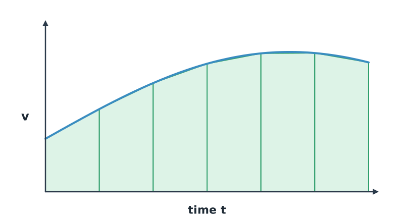
The trapezoidal rule

With sampled data, approximate the area with trapezoid strips. Each strip’s area is the average of its two edges times its width:

\int_{a}^{b} f d t \approx k \sum \frac{f _{k} + f _{k + 1}}{2} Δ t

Example 4. Distance from velocity

Velocity recorded every 1 s is 0, 2, 4, 4, 3 m/s.

d \approx \frac{0 + 2}{2} + \frac{2 + 4}{2} + \frac{4 + 4}{2} + \frac{4 + 3}{2} = 1 + 3 + 4 + 3.5 = 11.5 m

Charge consumed

A drone’s current sensor computes “mAh used” as the integral of current, $Q = \int I d t$ , in exactly the same way.

Example 5. How much battery is left?

A drone hovers at 20 A for 6 minutes, then flies fast at 30 A for 3 minutes.

First phase $20 A \times 0.1 h = 2.0$ Ah
Second phase $30 A \times 0.05 h = 1.5$ Ah
Total 3.5 Ah, or 3500 mAh

With a 5000 mAh battery and an 80% usage limit of 4000 mAh, only 500 mAh remain: time to fly home.

Why an IMU alone cannot navigate for long

An accelerometer measures acceleration. Integrate once for velocity, again for position, and it seems you could navigate without GNSS. But real sensors have a small constant offset called bias ( $b$ ). After two integrations, the position error grows with the square of time:

e (t) = \frac{1}{2} b t^{2}

Example 6. A tiny bias

A bias of $b = 0.05$ m/s² looks tiny, but after 60 seconds the position error is $\frac{1}{2} (0.05) (6 0^{2}) = 90$ m.

This is why autopilots fuse IMU data with GNSS, barometer or camera data using a Kalman filter (EKF), which you will study in DRT 335.

Common mistakes

Watch out

Confusing average and instantaneous velocity.
Forgetting time units. With current in A and time in minutes, convert to hours before getting Ah.
Differentiating noisy data without filtering.
Assuming integration error grows linearly. It grows with the square of time.

Summary

The derivative is the instantaneous rate of change, equal to the slope of the tangent.
Velocity is the derivative of position and acceleration the derivative of velocity; the power rule is $d (t^{n}) / d t = n t^{n - 1}$ .
Maxima and minima occur where the derivative is zero.
The integral is accumulation, the area under a graph; with real data, use the trapezoidal rule.
Charge used is the integral of current, and IMU bias causes position error of $\frac{1}{2} b t^{2}$ .

Check your understanding

Differentiate $x (t) = 3 t^{3} - 4 t + 7$ .
A drone is at 20 m at $t = 2$ s and at 35 m at $t = 5$ s. What is its average velocity?
Find when $h (t) = 8 t - 2 t^{2}$ is at its maximum, and the maximum value.
Current logged every 60 s is 18, 22, 20 A. Estimate the charge used in mAh with the trapezoidal rule.
An IMU has a bias of 0.02 m/s². What is the position error after 30 s?

Answers

$x^{'} (t) = 9 t^{2} - 4$
$(35 - 20) / (5 - 2) = 5$ m/s
$h^{'} (t) = 8 - 4 t = 0 \Rightarrow t = 2$ s and $h (2) = 16 - 8 = 8$ m
$(\frac{18 + 22}{2} + \frac{22 + 20}{2}) \times 60 = 41 \times 60 = 2460$ A·s; divided by 3600 gives 0.683 Ah, about 683 mAh
$\frac{1}{2} (0.02) (3 0^{2}) = 9$ m

Key formulas

Average velocity	$v ˉ = \frac{Δ x}{Δ t}$
Derivative	$v (t) = \frac{d x}{d t} = lim_{Δ t \to 0} \frac{x ( t + Δ t ) - x ( t )}{Δ t}$
Power rule	$\frac{d}{d t} t^{n} = n t^{n - 1}$
Finite difference	$v_{k} \approx \frac{x _{k + 1} - x _{k}}{Δ t}$
Trapezoidal rule	$\int_{a}^{b} f d t \approx \sum_{k} \frac{f _{k} + f _{k + 1}}{2} Δ t$
Charge consumed	$Q = \int I d t$
Error from bias	$e (t) = \frac{1}{2} b t^{2}$

Key references

Strang, G., & Herman, E. (2016). Calculus volume 1. OpenStax. link
Stroud, K. A., & Booth, D. J. (2020). Engineering mathematics (8th ed.). Bloomsbury.
Groves, P. D. (2013). Principles of GNSS, inertial, and multisensor integrated navigation systems (2nd ed.). Artech House.

In class / field

Lecture, case discussion and in-class problem solving

Learning evidence: Quiz results and submitted exercises

Module quiz

This is a formative self-check, not a graded exam

Knowledge domain: Mathematics, physics and statistics · Automation, robotics and swarms · Control, autopilot and navigation

Elementary calculus of motion

By the end of this module you will be able to

The mathematics of change

Rate of change and the derivative

Average velocity

Instantaneous velocity

The power rule

Finding maxima and minima

Derivatives from real data

The integral: accumulation

The trapezoidal rule

Charge consumed

Why an IMU alone cannot navigate for long

Common mistakes

Summary

Check your understanding

Key formulas

Key references

Further reading

Derivatives, rates of change and numerical integration

Exercise: measuring trajectory error

In class / field

Module quiz

Elementary calculus of motion

Lesson

By the end of this module you will be able to

The mathematics of change

Rate of change and the derivative

Average velocity

Instantaneous velocity

The power rule

Finding maxima and minima

Derivatives from real data

The integral: accumulation

The trapezoidal rule

Charge consumed

Why an IMU alone cannot navigate for long

Common mistakes

Summary

Check your understanding

Key formulas

Key references

Further reading

Derivatives, rates of change and numerical integration

Exercise: measuring trajectory error

In class / field

Module quiz